Deeper Dive: Untangling Tasks in a Toy Transformer
Transformer models are notoriously black-box, making it difficult to see how a model’s neurons act together to make a certain decision or formulate a certain outcome. This has serious consequences for model safety: models can learn harmful tendencies that go beyond overfitting, such as giving grievously incorrect advice or answering unsafe queries (e.g., “Provide detailed instructions on how to build a nuclear bomb”). We can look inside our models to better understand model thinking and intervene to curb harmful neuronal pathways.
To play with this idea, we train a toy transformer capable of two tasks: addition, and concatenation, and set out with a simple goal: to disable or significantly hinder the model’s capability to do one task, but not the other. By using Sparse Autoencoders to induce sparsity, followed by ablation with PyTorch hooks, we successfully and significantly remove the function of our choosing, while leaving the unselected function almost entirely unaffected.
This is a sister article to “Untangling Tasks in a Toy Transformer”. This article is more technically complete and provides some of the motivations for certain architectural decisions. This serves as a deeper dive to someone more familiar with the traditional aspects of machine learning. As with the first article, the code is fully available on GitHub.
Configuration & Setup:
This project uses
NumPy
PyTorch
Matplotlib
Seaborn
Dataset:
Since we are working with a toy transformer, and our tasks are both fairly straightforward, we can generate our own dataset. In this particular example, we want to train our model to handle concatenation and summation between two one-digit or two-digit numbers. We will represent each operation with either a “+” to denote addition, or a “C” to denote concatenation. We can then iterate through every combination of numbers from 0–99 inclusive to generate 10,000 pairs of prompt-and-answer examples for both tasks. We will prepend each example with a “B”, which will serve as a BOS token, and append each example with an “E”, which will serve as an EOS token. Finally, we want to ensure that all of our examples are the same length so that we do not have any shape irregularities while batching and training, so we pad all of our examples up to a length of 8, with a standard space (“ “) serving as our padding and mask token. This leaves us with a total of 20,000 examples.
We want to be able to tokenize our examples, and to facilitate training, we want to be able to batch our examples through PyTorch’s dataloader. We create a wrapper around PyTorch’s Dataset module, which we will call “StringDataset”. This class should be initialized as a PyTorch custom dataset. Our StringDataset’s “getitem” function should not tokenize via standard string to integer conversion, but should instead use maximal munch parsing.
Our use of maximal munch parsing here is semi-principled. Modern tokenizers provide a more efficient tokenization than simple string to integer, dictionary-style tokenization, often by combining several characters into single tokens. Practically, we see a substantial performance increase provided over earlier attempts at the model architecture (without maximal munch, val loss hovered around ~1–3, compare to ~0.1 now). This discovery was unintentional: In a now unused and unincluded portion of this project, attempts at activation patching were difficult to draw meaningful conclusions from, as comparing addition and concatenation would require at least looking at multiple tokens. As an example, “B7+7E” -> “B14E”, “B7C7E” -> “B77E” would require a comparison between “1”, “4”, “7”, and “7”, which quickly became too tedious to establish any general meaning across many examples. With maximal munch parsing, this would just be a comparison of “14” and “77”. Despite the activation patching approach ultimately being unused, it was this simplification attempt which revealed the performance improvements of maximal munch parsing.
Now, we need to create our training and validation datasets. Here, we borrow the train/val split decision from Nanda et al.’s progress measures for grokking paper, which trained a toy transformer to generalize to understand modular arithmetic. This paper split their dataset to avoid model memorization, with 30% of the examples used to train, and 70% to be used as validation data. We enable shuffling on the training set, and load our datasets into Torch dataloaders with a batch size of 512. We follow the same split, and (optionally) use pickle to save our train and validation datasets.
Model & Training Architecture:
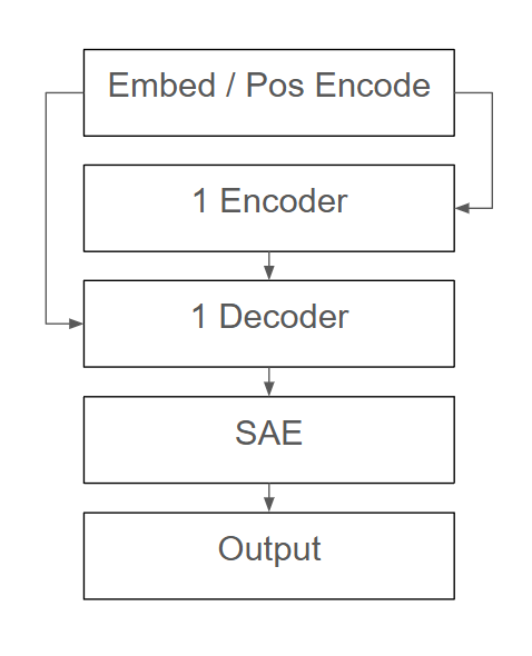
Our model architecture consists of a standard single-layer transformer encoder-decoder pair, followed by a sparse auto-encoder block. Originally, the architecture consisted of a single decoder block, which aimed to make the analysis of features as simple as possible. However, this was not sufficiently performant, so opting for a translation-like task architecture meant including the encoder. The architecture now contained two blocks, which made direct ablation of neurons in these blocks infeasible for quick intuition building. Looking at the cross-attention between the two blocks, or any attention patterns, was not explored in this example, as attention is not sufficient to serve as explanation for our underlying model thinking. Before modifying the model architecture further, an attempt was made to detect consistent attribution patterns with Captum, which did not reveal any consistent differences in neuron attribution between addition and concatenation examples, meaning we could not rely on these attributions to ablate our features precisely.
The final modification to the architecture was the addition of the sparse auto-encoder component, which greatly simplified the ablation task. The sparse auto-encoder is a simple up-project (4 times residual stream dim), non-linearity (ReLU), and down-project (back to residual stream dim), but comes with two powerful regularization parameters: MSE Alpha, which controls reconstruction loss penalty, and L1 Lambda, which controls sparsity.
The MSE Alpha parameter (which we set to its maximum value in training, 1), controls the importance of our sparse autoencoder in adequately replicating the previous layers. This is significant: assuming our sparse autoencoder achieves minimal reconstruction loss, we can represent the entirety of our model in a single block, which removes the burden of the larger search space of both encoder and decoder. This also means that the SAE is an excellent proxy for ablations in general, as deleting important activations in the SAE allows us to make changes across multiple blocks, bypassing the need to find multi-layer/block combinations of neurons that produce a certain result. Importantly, this allows us to make broad non-linear modifications to our model with simple linear modification to SAE neurons, and to directly assess the loss to see whether our modification had the desired effect.
The L1 Lambda parameter also supports our ablation goals, as it drives an increase of sparsity of our SAE. This functions as a standard regularization parameter, penalizing neurons with overly high magnitudes, which prevents the sparse auto-encoder from using a single neuron to accomplish multiple tasks. This helps our SAE avoid polysemanticity, or the overlapping of model functions/thinking on a single neuron. Naturally, the additional sparsity is great for understanding how our model works, but this is especially important if we want to make surgical trims to one of our features without damaging the other. The closer the value is to 1, the higher sparsity is forced to be, which can sometimes compete with accurate reconstruction. We use a value of 0.001 for this parameter.
It is also important to point out that our SAE is not trained post-hoc, that is, we train our model alongside our SAE instead of freezing our model and training the SAE afterwards. This is a bit unusual; in fact, using this same architecture and training the SAE separately from the model actually confers better loss performance during training. However, when the SAE was trained separately from the main model architecture, neuron ablations would typically break both tasks, even if the neuron was not identified in causing loss increase or having any activations in the task to be preserved. This seems to suggest that the SAE’s post-hoc training might still be effective in reducing polysemanticity, instead opting for the formation of circuits, or multi-neuron pathways, which are not apparent when iterating through individual neurons. Consequently, the presence of circuits makes straightforward ablation difficult for our demonstration, so we opt to train our SAE with the rest of our model instead.
We select a fairly high learning rate of 0.001, alongside 1000 epochs for training. These are generally sufficient to achieve a performant model (~0.1 best val loss), although there is some minor inconsistency between model runs. CV could be applied here to determine the extent of this. Transformer blocks are initialized with 4 heads, dim 256, and MLP up projection dim 4*256.
The final interesting component of our architecture and training parameters is our weight decay, which we also borrow from Nanda et al. We set our weight decay to 1, causing our model to aggressively forget. Intuitively, this practice applies a high penalization for the memorization of examples, in hopes that the model will instead find it more loss-efficient to learn the underlying pattern or relationship of the data rather than relying on memory. Since we wish to ablate the model’s ability to do addition and concatenation, we want to ensure that the model adequately learns these functions and develops an underlying pattern for both examples so that we would be able to adequately disrupt it at will. Assuming our model does, in fact, learn the underlying relationship of our functions, this would also make our SAE and neuron analysis more meaningfully interpretable.
Our high weight decay can induce instability during training, but helps our model converge faster. To improve training stability, we can set our weight decay to 0.5 and double our epochs to 2000.
Training:
We combine all of these concepts in our training loop. Our training will be done on the GPU, so we begin by sending our model there. Our optimizer will be AdamW, initialized with our model params, lr, and weight decay.
For every epoch, we iterate through our train dataloader, and send our prompts and answers to our GPU (to be on the same device as our model). For every pair of prompts and answers, we first zero out our optimizer. We call our model for our forward pass, and input both our prompt, and our target answer, to our model. Since our model was initialized with a Sparse Autoencoder, our model outputs logits, a prediction, as well as a reconstructed prediction and the SAE’s sparse activations. We begin by taking the cross entropy loss between our logits and our target answer, then we take the MSE loss between our original predictions and our SAE-reconstructed predictions, and then we take the norm of our sparse activations followed by a mean.
We combine these loss modalities into a single loss function,
Loss = Cross Entropy Loss + (MSE_Alpha * MSE Loss) + (L1_Lambda * Mean Norm Sparse Activations)
And then calculate our backwards pass from this loss. Optionally, we norm clip our gradients to avoid explosive gradients. Finally, we step with our optimizer, and after the end of an epoch, we calculate our total loss for our train set. To assess how our model fares on our validation set, we switch the model into eval mode to prevent gradient calculations, and repeat the process with our validation data sans running a backward pass. We record the best validation performance. If a model has the best validation performance, then we save the checkpoint of the model at that epoch, overwriting any previous saved model.
To initiate training, we can first define our model by calling its class, including an argument about the size of our tokenizer dictionary, so that the model can initialize its embedding and output matrices. Then, we run the training function we defined.
Model Performance & Prediction:
Our model is performant. We can use our model by switching it into eval mode, and providing our prompt, along with a single beginning of sentence token to have the model complete the rest. Performance, however, can be variable, even when all the same parameters are passed. CV, as well as different val/train split ratios, should be performed on this model to determine how performance changes, and what steps can be taken to stabilize the model.
Performance decreases if the learning rate is changed higher or lower.
The following results are representative of the typical model trained:
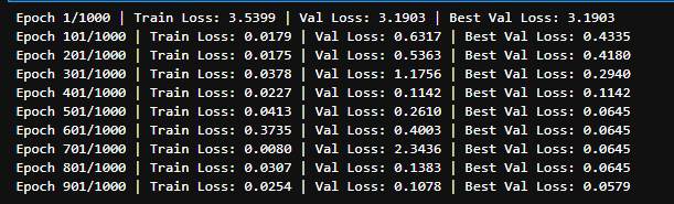
And on a random sample of 1000 question/answer combinations from the validation set passed through the model,
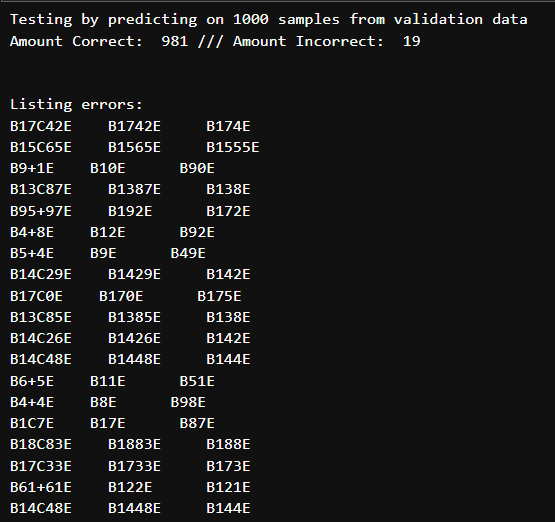
We see that 98.1% of all of our predictions are correct. The prompt is on the left, the true answer in the middle, and the prediction on the right. In most of the models trained, there appears to be some small pattern in the incorrect predictions. Interestingly, most of the incorrect predictions are not wildly incorrect, and are almost always off by only a single digit.
Assessing Sparsity:
Now that we have a performant model, we can be more certain of the credibility that interpreting this model presents us, as well as the meaningfulness of our ablations. Before we can begin ablating our neurons, we want to assess how well our regularization term sparsified our SAE.
We can define a function that places PyTorch hooks on our encoder, decoder, and our SAE encoder and decoder. This function will record the activations for a particular specified block. We then pass a sample prompt-answer pair, our PyTorch hooks record our activations, and then we specifically remove our PyTorch hooks (so as to not damage the model) before moving on and visualizing the activations we collected.
We see that we successfully induced sparsity in our SAE, with most activations being 0.
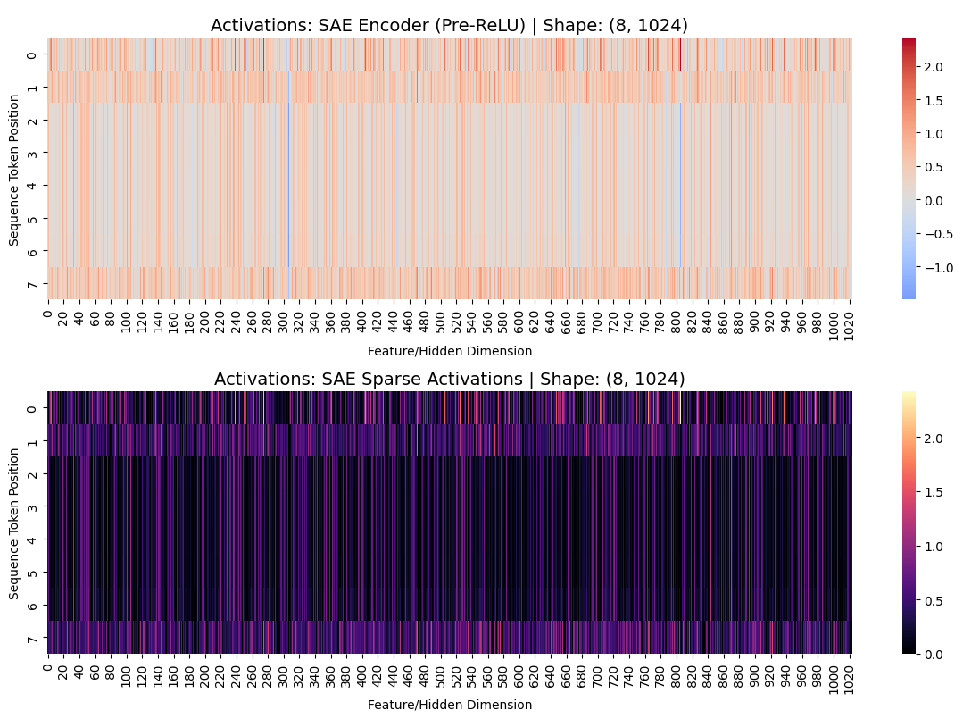
SAE L1 Lambda = 0, i.e. model trained with no sparsity term. 97% of post-ReLU sparse activations are non-zero.
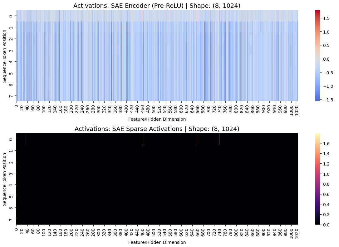
SAE L1 Lambda = 0.01, i.e. model trained with strong sparsity term. 0.1% of post-ReLU sparse activations are non-zero.
Determining Neuron Importance:
We can determine the importance of our neurons by assessing how much our loss changes when we zero-ablate a particular neuron. Conceptually, we would want to do this for multiple addition and concatenation examples to determine whether we see any neurons that consistently activate for one task, but not the other. To ensure that our examples are as similar as possible, differing only in what operation is used in the prompt (and, naturally, in their answer), we can select addition examples from our validation dataset, generate concatenation examples from them (by changing the operation symbol used, and the answer), and then assess whether those concatenation examples are in the training set. Finally, once we have discarded any examples where the concatenation example is in our training set, we can see whether the model accurately predicts the examples. Any example incorrectly predicted is also discarded.
Once we have our final set of examples, we can pass each one through, and determine which neurons are, on average, responsible for the greatest increase in loss on both the summation and concatenation examples.
Ablation Results:
Now that we know which neurons are important to each task, we can, at this point, attempt to remove the function of either addition or concatenation simply by removing the neurons that activate most strongly for that task. Although our sparsity regularization may have been successful in reducing some polysemanticity, it is possible that quite a few features are still modulated by the same neurons.
The most basic counter to this problem is comparing each neuron’s average scores, and, once we have determined which task we want to ablate, we can remove the neurons that are responsible for that task only, i.e. those that have no importance or loss increase on the task we wish to preserve. This approach, while safe, often leads to fairly unimpressive, (and depending on the model and choice of samples, variable), results. Generally, we can expect to see a 4–12% drop in the task we wish to ablate, with complete preservation of the other task.
This may seem like our approach has failed entirely. However, our decision to add a sparsity inducing term has partially rescued us here: although some amount of polysemanticity still remains, neurons which contain relevance to both features are generally much more relevant to one feature than the other. If we are willing to accept some minimal loss in the task we wish to preserve in exchange for the near-total removal of the other task, then we would have successfully achieved our goals.
We can accomplish this through the introduction of a tolerance parameter, which allows us to specify how much loss we are willing to accept in our task-to-be-preserved per neuron. We write our ablation function such that we will never ablate a neuron if it is more important in the task-to-be-preserved than in our task-to-be-ablated.
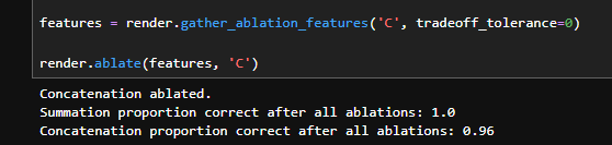
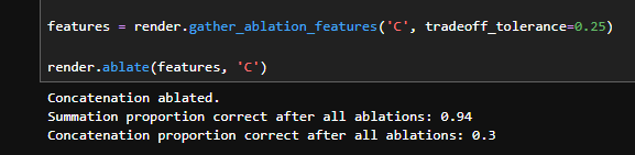
With the addition of the ablation parameter, we see that we are able to make small performance tradeoffs in the feature that we wish to preserve in exchange for massive performance decreases in the feature that we wish to ablate. Whereas the approach without a tolerance parameter conferred a 4–12% drop in the proportion correct of the ablated task, using the tolerance parameter typically sacrifices 5–15% of the preserved task’s performance in exchange for 70–90% loss of function in the ablated task. Furthermore, the ablation parameter allows for manual control of the tradeoff, and more or less can be sacrificed depending on the sufficiency of unwanted task ablation.
We see that this is a viable approach to delete tasks in a toy model! Although we did not get complete separation of our tasks, this is still likely achievable with the correct balance of learning rate and L1 Lambda parameter. Additionally, this project borrowed several concepts from the grokking Nanda et al. paper, particularly high weight decay choice and train/test split decision. Our model did not grok; we actually achieve fairly consistent improvements in our validation set loss, however, we retain these borrowed concepts because they worked well for this architecture and make sense spiritually. Finally, we see irregularity between our model runs. This is most likely caused by the weight decay parameter, which can be modified proportionally to the amount of epochs: halving our weight decay means doubling our epochs. It could be worthwhile to train the model with cross validation to understand how much the model performance differs based on the data it is trained on.
In short, there are many low-hanging improvements to be made on this toy model demonstration. Hopefully, we can use interventions like these to improve our understanding of our models as we build towards AI safety.