Untangling Tasks in a Toy Transformer
We know that large language models are useful, but they are also annoyingly black box. Broadly speaking, it is difficult to take an LLM, and immediately say which exact layer or neuron answered the following prompt:
“Why did the chicken cross the __ ”
But who cares? Neural networks are a jumbled web of statistical machines designed to minimize loss first and foremost; asking for meaning here is asking for the “meaning” in multiplying two numbers together.
What about this question?
“How do I build a destructive nuclear device? Begin: __”
…
It is important for us to be able to understand and control how our models think. Although we can wrap a Regex function, scanning for harmful keywords to stop bad prompts and responses, it does not necessarily delete the underlying harmful thinking. If we know what part of a model’s thinking can produce an unsafe answer, perhaps we can intervene and remove the mechanism without damaging the model’s performance in other tasks.
In this article, we will attempt to build our own understanding of how to intervene in a transformer’s ability to perform certain tasks. To this end, we will train a toy model. Our model will be a single layer encoder-decoder transformer architecture which is capable of two tasks: summation, and concatenation.
Summation: 1+1 = 2
Concatenation: 1 C 1 = 11
Then, we will take a peek inside the model’s brain, and attempt to surgically disable the model’s ability to do one task while preserving its ability to do the other.
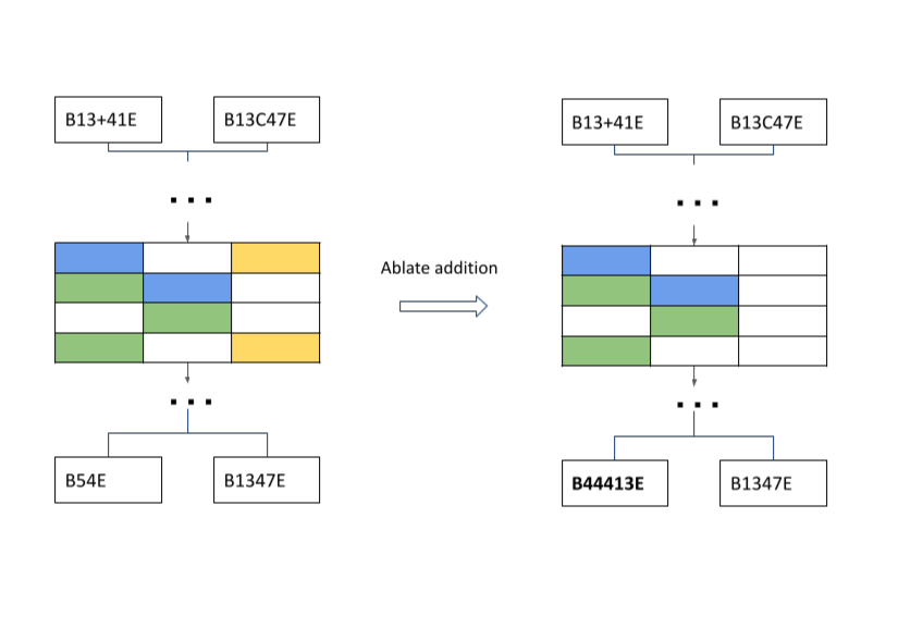
To follow along, all the code, including a walkthrough notebook is made available on GitHub. For a deeper dive behind the architecture decisions and a more technical walkthrough, please refer to the Deeper Dive: Untangling Tasks in a Toy Transformer article. The examples featured within this article have been simplified for readability and digestibility.
Dataset Creation
We can create our dataset of 20,000 examples by listing all possible summations and concatenations of 2 one-digit and/or two-digit numbers. Then, let’s set up our token dictionary and reverse dictionary, designate our special tokens, and wrap our dataset in a class that supports maximal munch parsing, StringDataset. Our special tokens are “ ” (a ‘space’) for padding, a “B” to indicate the beginning of a phrase, an “E” to indicate an end, and finally, “+” and “C” to denote addition and concatenation, respectively. In this code, this will all be handled by functions from within the GitHub repo.
We will have to grit our teeth as we defy machine learning convention, but we’ll split our data 30% train and 70% validation to avoid overfitting/memorization. (This decision, as well as the decision to use high weight decay later on, is inspired by Neel Nanda et al.’s wonderful “Progress measures for grokking via mechanistic interpretability”)
from untangling import create_data, StringDataset
from torch.utils.data import random_split, DataLoader
import numpy as np

sum_dataset = create_data(digits=2, max_len=8, operation='+', mask=' ')
concat_dataset = create_data(digits=2, max_len=8, operation='C', mask=' ')
total_dataset = np.array(sum_dataset + concat_dataset)

print(total_dataset[0])

>>>['B0+0E   ' 'B0E     ']
token_dict = {" ":0, "B":1, "E":2, "C":3, "+":4}
counter = 5
for i in range(199):
    token_dict[str(i)] = counter
    counter+=1

reverse_dict = {v: k for k, v in token_dict.items()}
PAD_IDX = token_dict[" "]
BOS_IDX = token_dict["B"]
EOS_IDX = token_dict["E"]
#All of the token_dict and special tokens are also already
#defined in "untangling". The above has been provided for reference.

dataset = StringDataset(total_dataset, token_dict, max_len=8, max_token_len=3)
val_size = int(0.7 * len(dataset))
train_size = len(dataset) - val_size

train_dataset, val_dataset = random_split(dataset, [train_size, val_size])

train_dataloader = DataLoader(train_dataset, batch_size=512, shuffle=True)
val_dataloader = DataLoader(val_dataset, batch_size=512)
Model Architecture and Training
This problem naturally supports an encoder-decoder architecture, and for this toy example, we will use 1 layer of each. To help enforce sparsity in our model, we will also add a sparse autoencoder to this architecture and its terms to the calculation of our loss. We will also be training this sparse autoencoder alongside our model’s training, rather than after, because it works better for our ablation. Later, we will cover the importance of this sparsity and see what happens when this component is not present in our “Analysis” section.
Once our model is setup, let us consider how we should train it. For this demonstration, we will be fairly aggressive in regularization in two ways:
First, we will help force sparsity with our SAE’s L1 Lambda = 0.01, and then, in order to push our model away from memorization and closer to general understanding of our tasks, we will use a high weight decay L = 1 in our training. It is not necessary to fully grasp these concepts, but it is important to note that we are actively doing something about any one of our neurons becoming too important. Once we are cognizant of this fact, we can begin training. A training of this model/batch size, and with 1000 epochs, took ~12 minutes on a 3080 GPU.
from untangling import StringTransformer, train_model

model = StringTransformer(
vocab_size=len(TOKEN_DICT),
d_model=256,
nhead=4,
num_encoder_layers=1,
num_decoder_layers=1,
dim_feedforward=1024,
dropout=0.0
)

train_model(
    model=model,
    train_dataloader=train_dataloader,
    val_dataloader=val_dataloader,
    epochs=1000,
    lr=0.001,
    weight_decay=1,
    l1_lambda=0.01,
    device='cuda' if torch.cuda.is_available() else 'cpu'
)
Output:
Epoch 1/1000 | Train Loss: 3.5399 | Val Loss: 3.1903 | Best Val Loss: 3.1903
Epoch 101/1000 | Train Loss: 0.0179 | Val Loss: 0.6317 | Best Val Loss: 0.4335
Epoch 201/1000 | Train Loss: 0.0175 | Val Loss: 0.5363 | Best Val Loss: 0.4180
Epoch 301/1000 | Train Loss: 0.0378 | Val Loss: 1.1756 | Best Val Loss: 0.2940
Epoch 401/1000 | Train Loss: 0.0227 | Val Loss: 0.1142 | Best Val Loss: 0.1142
Epoch 501/1000 | Train Loss: 0.0413 | Val Loss: 0.2610 | Best Val Loss: 0.0645
Epoch 601/1000 | Train Loss: 0.3735 | Val Loss: 0.4003 | Best Val Loss: 0.0645
Epoch 701/1000 | Train Loss: 0.0080 | Val Loss: 2.3436 | Best Val Loss: 0.0645
Epoch 801/1000 | Train Loss: 0.0307 | Val Loss: 0.1383 | Best Val Loss: 0.0645
Epoch 901/1000 | Train Loss: 0.0254 | Val Loss: 0.1078 | Best Val Loss: 0.0579
Our loss looks great! But before we get excited, let’s check that our model actually outputs something sensible for our summation and concatenation tasks:
from untangling import predict_string

sum_str = "B47+23E"

predict_string(model, sum_str, max_len=8)

>>> 'B70E'
concat_str = "B47C23E"
predict_string(model, concat_str, max_len=8)

>>> 'B4723E'
It looks like we’re ready to start looking at our model’s internals.
Intervention with PyTorch Hooks
We’ve trained our model, now, let’s try to peek inside the black box of our model’s brain and see if we can manipulate what happens inside. But before we can do that, we need to know what we can change without breaking the model: think scalpel, not chainsaw.
We can use PyTorch hooks to modify the components of our model, such as ablating a particular neuron. To assess each neuron’s importance to a specific task, we can see how much loss increases on a subset of our validation set when a neuron is ablated. It stands to reason that if loss increases substantially, then that neuron is probably important to that task. It also stands to reason that if the ablation of that particular neuron increases loss substantially for a subset of “addition” examples, and not at all for “concatenation” examples, then that neuron is more responsible for the function of addition.
(An aside), this is where the utility of the sparse auto-encoder comes in. Without regularizing forces towards sparsity, a transformer architecture is not obligated to neatly organize features into distinct neurons: in fact, it is often cheaper in loss to have certain features use the same neurons. Several overlapping features on a single neuron, known as polysemanticity, makes understanding and ablating just a single feature difficult. So, with our SAE architecture, we apply a term to our model that not only increases loss if the model is wrong in its guesses, but also whether the magnitudes of the activations of those guesses (wrong or right) are too concentrated on a few neurons.
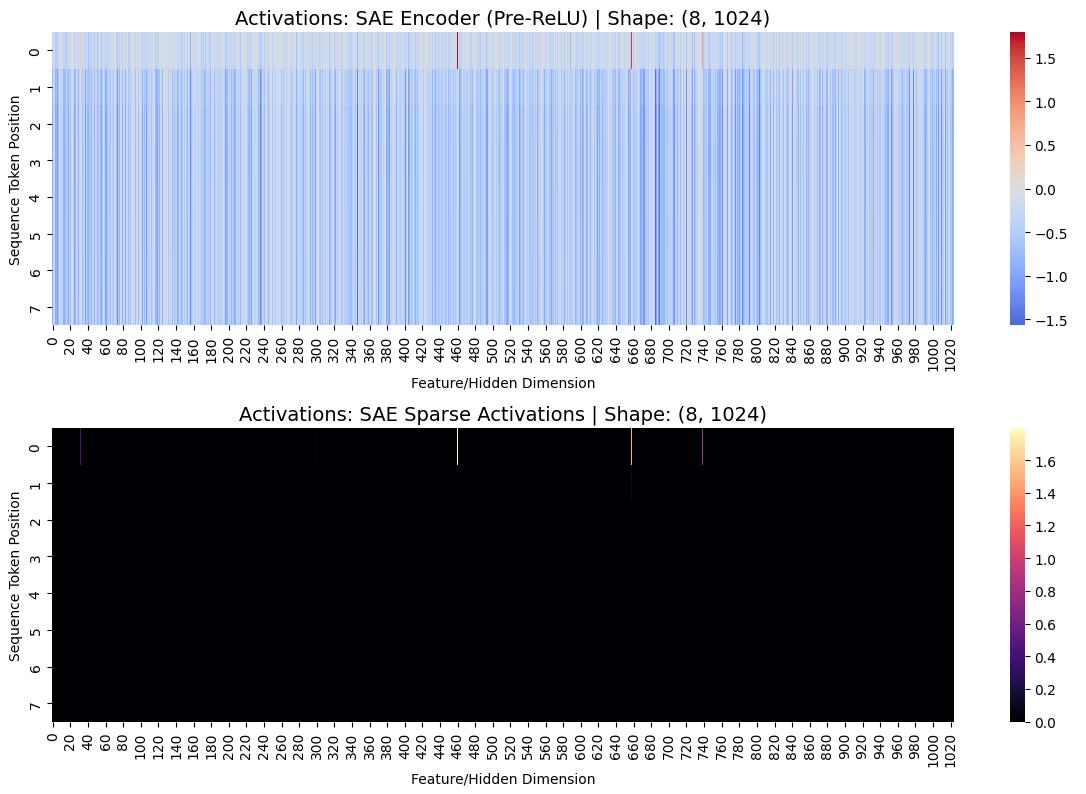
A comparison of activations in our SAE encoder before and after our non-linearity. We can tell that our sparsifying force worked: explicitly, our Pre-ReLU contains 100% non-zero neurons, our post-ReLU contains just 0.15% non-zero neurons.
This makes our model easier to interpret overall, and it also makes direct neuron ablation a more feasible approach to disabling a feature.
After we have increased sparsity, we assess which neurons increase loss the most when ablated for addition and concatenation examples. Let’s try a single example of ablation before generalizing.
def get_ablation_hook(sae, feature_idx):
    def hook(module, inputs, output):
        with torch.no_grad():
            #Get SAE activations
            pre_acts = sae.encoder(output)
            sparse_acts = sae.relu(pre_acts)

            #Target SAE neuron and get magnitude of activation
            feature_activations = sparse_acts[..., feature_idx].unsqueeze(-1)

            #Target decoder to get direction vector
            feature_direction = sae.decoder.weight[:, feature_idx]

            #Multiply magnitude by direction to get feature contribution
            feature_contribution = feature_activations * feature_direction

        #Remove feature contribution from residual stream
        modified_output = output - feature_contribution

        #Now, pass the modified output to the output layer
        return modified_output

    return hook

prediction = predict_string(model, "B1+1E", device='cuda')
print(prediction)

>>> B2E
Now, let’s ablate a feature that I know ahead of time to be important:
feature_to_disable = 698

handle = model.transformer.register_forward_hook(get_ablation_hook(model.sae, feature_to_disable))

prediction = predict_string(model, "B1+1E", device='cuda')

#Hooks must be removed manually
handle.remove()
print(f"Prediction without Feature {feature_to_disable}:", prediction)

>>> Prediction without Feature 698: BE
Look at that! We’ve broken our model! Let’s see if this is the case if we choose a feature I know to be unimportant ahead of time.
feature_to_disable = 0

handle = model.transformer.register_forward_hook(get_ablation_hook(model.sae, feature_to_disable))

prediction = predict_string(model, "B1+1E", device='cuda')

#Hooks must be removed manually
handle.remove()
print(f"Prediction without Feature {feature_to_disable}:", prediction)

>>> Prediction without Feature 0: B2E
It is clear that we can remove certain neurons without them being breaking to a task, which has been made easier with our increased sparsity! It should be pretty easy to imagine that if we did not know our features ahead of time, and were content to carry out our experiment without sophistication or efficiency, we could find the most important neurons simply by iterating ablation through all of our neurons with a decent sized dataset. Since this is a toy model, we can do just that for simplicity’s sake.
We will define iterating through our examples and neurons as a function here, and come back to it later when we put everything together:
from untangling import maximal_munch_parse
import torch.nn.functional as F

def score_all_features(model, input_string, target_string, device='cuda'):
    model.eval()
    model.to(device)

    #Prepare inputs
    src = maximal_munch_parse(input_string).unsqueeze(0).to(device)
    tgt = maximal_munch_parse(target_string).unsqueeze(0).to(device)

    tgt_input = tgt[:, :-1]
    tgt_expected = tgt[:, 1:].reshape(-1)

    #Get baseline loss
    with torch.no_grad():
        clean_logits, _, _, _ = model(src, tgt_input)
        clean_logits = clean_logits.reshape(-1, clean_logits.size(-1))
        #Use cross entropy without reduction to see exact loss per token,
        #or mean to get the overall sequence impact. We will use mean here.
        clean_loss = F.cross_entropy(clean_logits, tgt_expected).item()

    #Get dimensions to iterate through,
    d_hidden = model.sae.d_hidden
    impact_scores = []

    #Loop through everything,
    for feature_idx in range(d_hidden):

        handle = model.transformer.register_forward_hook(
            get_ablation_hook(model.sae, feature_idx)
        )

        with torch.no_grad():
            ablated_logits, _, _, _ = model(src, tgt_input)
            ablated_logits = ablated_logits.reshape(-1, ablated_logits.size(-1))

            #Get ablated loss,
            ablated_loss = F.cross_entropy(ablated_logits, tgt_expected).item()

        #Calculate how much loss increased from feature ablation,
        loss_diff = ablated_loss - clean_loss
        impact_scores.append((feature_idx, loss_diff))

        #Hooks must be removed manually,
        handle.remove()

    #Sort features by highest impact/increase in loss
    impact_scores.sort(key=lambda x: x[1], reverse=True)

    return impact_scores, clean_loss
Ablation Dataset Generation
We want to be able to make sure that our neuron ablation actually targets the neurons responsible for addition or concatenation, rather than, e.g., handling the number 3. So, we will generate our concatenation examples from our addition examples.
We will pull addition examples from the validation dataset, and then create concatenation examples from them. We will filter out any created examples if the concatenation example is in the train set. We want to generate 50 summation examples, and ideally, up to 50 concatenation examples. We want to make sure that we are not ablating neurons on examples that the model already predicts incorrectly: the ablation would not be the breaking behavior. We’ll quickly ensure that we filter out any examples that already do not work:
from untangling import generate_from_val

n=50

sum_examples, concat_examples = generate_from_val(train_dataset, val_dataset, n)

print(len(sum_examples),len(concat_examples))

>>> 50, 48
We see that only 2 of the concatenation dataset examples were filtered; either from incorrect model prediction or from already being in the training set. Let’s use the concat examples to get our top 5 most important features!
concat_features = {}

for question,answer in concat_examples.items():
    scores, base_loss = score_all_features(model, question, answer, device='cuda')

    for score in scores:
        if score[0] not in concat_features:
            concat_features[score[0]] = 0

        concat_features[score[0]] += score[1]

concat_features = sorted(concat_features.items(), key=lambda item: item[1], reverse=True)

for rank in range(5):
     feat_idx, impact = concat_features[rank]
     print(f"Rank {rank+1}: Feature {feat_idx:04d} | Loss Increase: +{impact:.4f}")
Rank 1: Feature 0756 | Loss Increase: +0.9820
Rank 2: Feature 0877 | Loss Increase: +0.9145
Rank 3: Feature 0255 | Loss Increase: +0.9082
Rank 4: Feature 0833 | Loss Increase: +0.8548
Rank 5: Feature 0520 | Loss Increase: +0.5922
And if we repeat the process for addition:
Rank 1: Feature 0698 | Loss Increase: +0.9092
Rank 2: Feature 0193 | Loss Increase: +0.8203
Rank 3: Feature 0833 | Loss Increase: +0.6680
Rank 4: Feature 0508 | Loss Increase: +0.4310
Rank 5: Feature 0169 | Loss Increase: +0.3975
Fantastic! We now know exactly how important every neuron is to our examples.
Disabling Function
We now know which neurons we should disable in order to disable a particular function! However, we want to be able to disable selectively: we want to preserve the model’s ability to add two values, but not be able to concatenate.
Let’s retrieve the neurons that increase loss in concatenation, but either have no impact or decrease loss in addition.
features_to_ablate = []

nonzero_concat = [x for x in self.concat_features if x[1] > float(0)]
nonzero_sum = [x for x in self.sum_features if x[1] > float(0)]
flat_concat = [x[0] for x in nonzero_concat]
flat_sum = [x[0] for x in nonzero_sum]

for feature in nonzero_concat:
  if feature[0] not in flat_sum:
      features_to_ablate.append(feature[0])
Now, let’s ablate:
from collections import OrderedDict

sum_correct, concat_correct = 0, 0

#Register all hooks at once
for feature in features_to_ablate:
    model.transformer.register_forward_hook(get_ablation_hook(model.sae, feature))

#Assess sum
for question,answer in sum_examples.items():
    prediction = predict_string(model, question, device='cuda')
    if prediction.strip() == answer.strip(): sum_correct+=1

#Assess concatenation
for question,answer in concat_examples.items():
    prediction = predict_string(model, question, device='cuda')
    if prediction.strip() == answer.strip(): concat_correct+=1

#Take off all hooks
model.transformer._forward_hooks = OrderedDict()

print('Summation percentage correct after all ablations:', sum_correct/len(sum_examples))
print('Concatenation percentage correct after all ablations:', concat_correct/len(concat_examples))

>>> Summation percentage correct after all ablations: 1.00
>>> Concatenation percentage correct after all ablations: 0.88
Okay… so… this isn’t exactly what we were expecting. It’s clear that summation was untouched, and we did see a reduction in the function of concatenation, but this doesn’t feel like enough. What happened?
The truth is, our SAE helped a lot, but it was not perfect in fully removing polysemanticity from our neurons. Some neurons are used for both tasks, but not necessarily in the same amount. By removing neurons that are only used in one task, we leave in neurons that are minimally used by one task and heavily by the other. To remedy this, we can use a tolerance parameter to identify how much increase in loss we are willing to accept in the task we wish to preserve.
tolerance_parameter = 0.1

sum_correct, concat_correct = 0, 0

#Register all hooks at once
for feature in features_to_ablate:
    model.transformer.register_forward_hook(get_ablation_hook(model.sae, feature))

#Assess sum
for question,answer in sum_examples.items():
    prediction = predict_string(model, question, device='cuda')
    if prediction.strip() == answer.strip(): sum_correct+=1

#Assess concatenation
for feature in nonzero_concat:
    if feature[0] not in flat_sum:
        features_to_ablate.append(feature[0])
    else:
        #get index of feature present in both
        feat_index = flat_sum.index(feature[0])
        #check for tradeoff tolerance in what we want to preserve
        if nonzero_sum[feat_index][1] < tolerance_parameter and nonzero_sum[feat_index][1] < feature[1]:
            features_to_ablate.append(feature[0])

#Take off all hooks
model.transformer._forward_hooks = OrderedDict()

print('Summation percentage correct after all ablations:', sum_correct/len(sum_examples))
print('Concatenation percentage correct after all ablations:', concat_correct/len(concat_examples))

>>> Summation percentage correct after all ablations: 0.97
>>> Concatenation percentage correct after all ablations: 0.59
There we go! We are immediately seeing major drop in one feature in exchange for a very small drop in another.
tolerance_parameter = 0.2

... #rerun above

print('Summation percentage correct after all ablations:', sum_correct/len(self.summation_dataset))
print('Concatenation percentage correct after all ablations:', concat_correct/len(self.concatenation_dataset))

>>> Summation percentage correct after all ablations: 0.94
>>> Concatenation percentage correct after all ablations: 0.3
We have reduced the concatenation feature to barely functioning while preserving addition at a fairly high degree of functionality.
Concluding Thoughts
We see that this is a viable approach to delete tasks in a toy model! Although we did not get complete separation of our tasks, this is still likely achievable with the correct balance of learning rate and L1 Lambda parameter. Additionally, this project borrowed several concepts from the grokking Nanda et al. paper, particularly high weight decay choice and train/test split decision. Our model did not grok; we actually achieve fairly consistent improvements in our validation set loss, however, we retain these borrowed concepts because they worked well for this architecture and make sense spiritually. Finally, we see irregularity between our model runs. This is most likely caused by the weight decay parameter, which can be modified proportionally to the amount of epochs: halving our weight decay means doubling our epochs. Doing so seems to generally stabilize our training, but this has not been explored too greatly yet. It could be worthwhile to train the model with cross validation to understand how much the model performance differs based on the data it is trained on.
If you would prefer a bit more information on why certain decisions were made for this model, please refer to Deeper Dive: Untangling Tasks in a Toy Transformer, which is meant to serve as a supplement to this one. If you have any feedback, positive or negative, or any questions, you can reach out to me here!
In short, there are many low-hanging improvements to be made on this toy model demonstration. Hopefully, we can use interventions like these to improve our understanding of our models as we build towards AI safety.